The Ogallala aquifer is on schedule. The schedule is a decline.
Testing whether the Ogallala under the Southern High Plains is falling no faster than its legal target, and how many wells it takes to know.
I’m no hydrogeologist. Just a fella with an interest in water and an internet connection. If you know this aquifer and something here looks off, I’d like to hear it.
I went into this expecting to find a Texas aquifer missing its conservation target. The Ogallala under the Southern High Plains has been pumped for irrigation since the 1940s, and it barely recharges. Surely the districts’ goals were not being met.
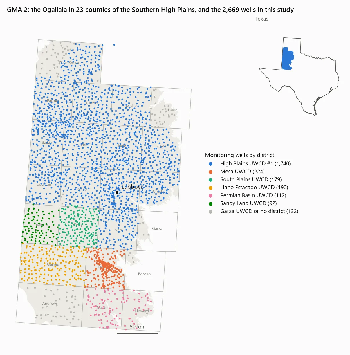
Then I read the goal. In Groundwater Management Area 2, the 23 counties around Lubbock, the groundwater districts’ desired future condition (DFC) for the Ogallala is an average water-level decline of 23 feet over sixty years. Eight of those feet are scheduled for the first decade. The target is a decline.
That turns out to be normal. Texas law asks the districts in each management area to pick a condition they want to protect, and the state converts it into a pumping budget. On an aquifer like the Ogallala, where little water comes back in, sustained pumping means falling levels, so in practice the question becomes how fast to draw it down. Elsewhere the targets look different. Parts of the Panhandle aim to keep 40% of their 2010 storage after fifty years. In Central Texas, the target is that Barton Springs keeps flowing at 6.5 cubic feet per second through a repeat of the 1950s drought. GMA 2’s target is simply a rate of decline.
So the question I could actually answer from public data was narrower:
Is the Ogallala in GMA 2 declining no faster than the agreed schedule, and how sure can we be?
It is, by about a foot
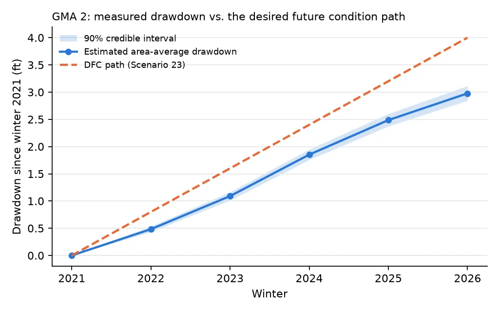
Between winter 2021 and winter 2026, the aquifer’s average water level fell 2.98 ft (90% credible interval 2.84 to 3.11). The schedule allowed 4.0 ft by now. On the data available, the model puts the probability that the aquifer is within its schedule above 99.9%.
| Winter | Allowed (ft) | Estimated decline (ft) | 90% interval |
|---|---|---|---|
| 2022 | 0.8 | 0.48 | 0.43-0.53 |
| 2023 | 1.6 | 1.09 | 1.01-1.17 |
| 2024 | 2.4 | 1.85 | 1.76-1.95 |
| 2025 | 3.2 | 2.49 | 2.37-2.60 |
| 2026 | 4.0 | 2.98 | 2.84-3.11 |
Before anyone hands out an award, a few things about that number.
The schedule was rewritten in 2026, and the rewrite matters. The previous DFC, adopted in 2016, allowed 23 to 27 ft of decline between 2012 and 2070. Spread evenly, that is about 0.4 ft a year. Against that schedule the aquifer is behind: 7.1 ft of decline since 2012, where an even pace allows 5.2 to 6.1.
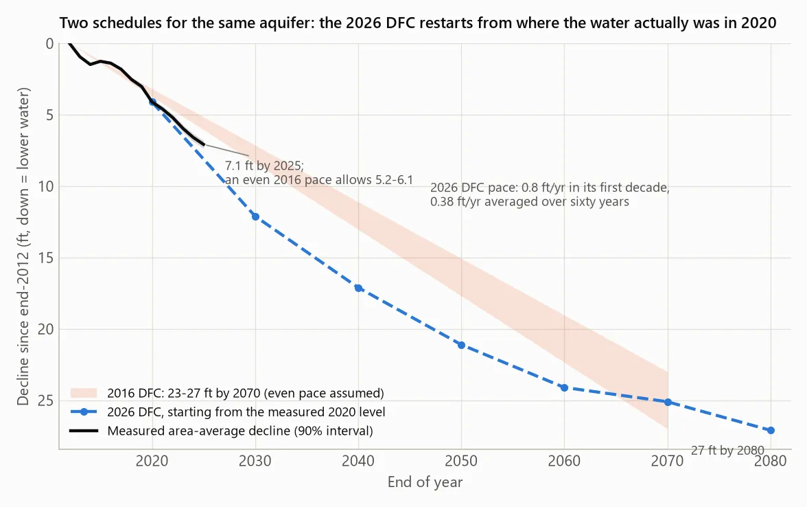
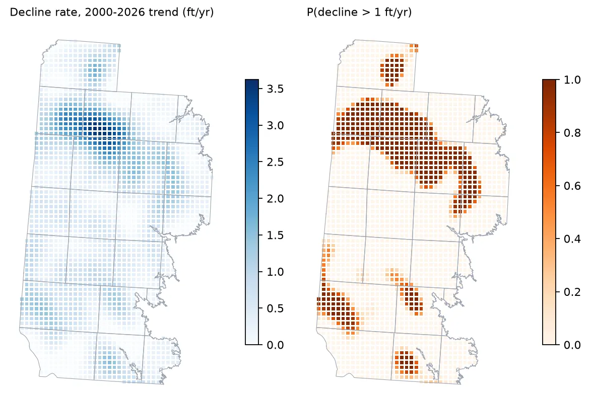
The new DFC doesn’t start from 2012. It starts from 2020, from wherever the water actually was, and lets the first decade carry 0.8 ft a year before slowing down. Put both schedules on the same axis and something interesting falls out. Add the 4.1 ft the aquifer had already lost by 2020 to the new DFC’s schedule, and it lands at about 25 ft by 2070, in the middle of the old 23-27 ft range. The destination barely moved. What changed is the pace: more decline allowed now, less later. The aquifer has been falling about 0.67 ft a year on average since 2000, so part of the reason it is on schedule seems to be that this decade is the most generous part of the schedule. The slower part, averaging about 0.3 ft a year from 2030 on, hasn’t started yet.
The DFC also gives each county its own number. As far as I can tell, these come from the groundwater model run behind the DFC, so they reflect where pumping is expected to be heaviest. Castro County, in the irrigated heart of the area, is allowed 9.5 ft of decline between 2021 and 2026. Lynn County, south of Lubbock, is allowed 2.0. The heavily irrigated counties have the largest allowances, and they are inside them: Castro fell 7.3 ft, Hale 4.7 ft against 9.0, and Lamb 5.1 ft against 6.5.
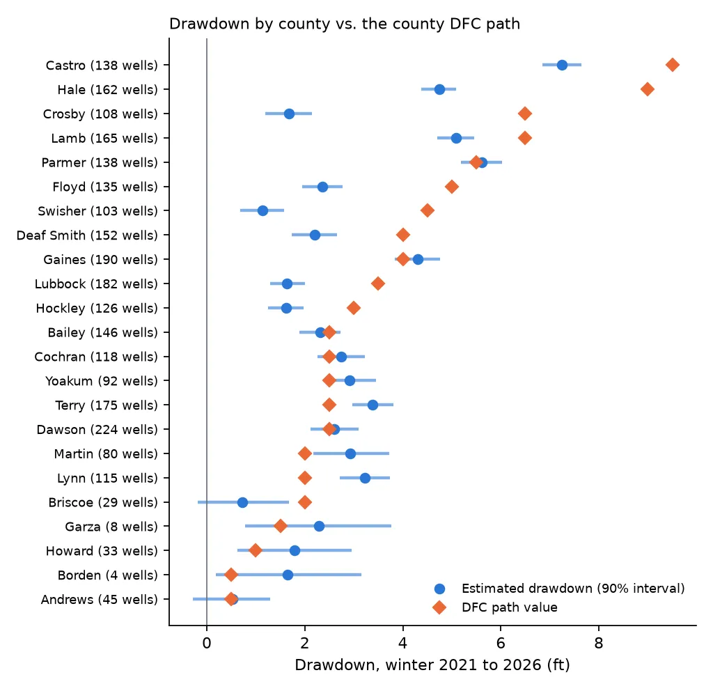
The counties that are over are in the south, where the allowances are small. Terry fell 3.4 ft against 2.5 and Lynn 3.2 against 2.0, and in both the model puts the chance of being within the allowance at essentially zero. Martin, at 2.9 against 2.0, is over with about 97% probability. Ten counties are clearly within their allowance. The other ten I can’t call either way at 90% confidence. Some of them have too few wells to say much (Borden has four, Garza eight), and others, like Gaines (4.3 ft against 4.0) and Parmer (5.6 against 5.5), sit almost exactly on the line.
Gaines is worth a sentence of its own, because an earlier version of the model called it over its allowance with 96% probability. That version looks to have been overconfident in the south, for reasons covered below. The corrected model gives Gaines a 13% chance of being within its allowance, which is a lean, not a call.
Where the data come from, and why a plain average is wrong
Every winter, after the irrigation season, the districts send crews out to measure water levels in about 1,800 wells. The measurements go into the Texas Water Development Board’s public groundwater database. I used every winter from 2000 to 2026: 2,669 wells with at least three winters, and 45,101 year-to-year changes, after dropping readings that disagree with themselves within a winter, wells whose recorded ground elevation is more than 50 ft off the national elevation model, and single-year spikes of more than 10 ft.
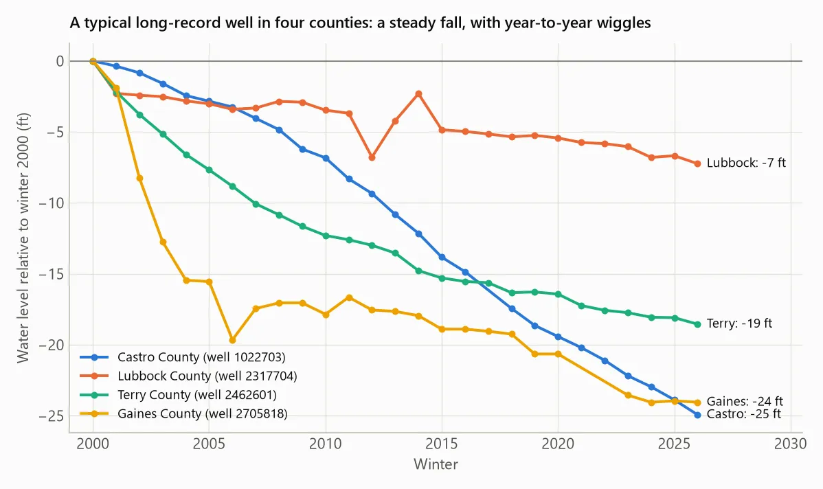
Individual wells tell the story at a glance. A typical well in Castro County, in the irrigated north, has lost 25 ft since 2000 at a nearly constant rate. One in Lubbock County has lost 7. Each line wiggles from year to year with the weather and with how hard the neighbours pumped that summer.
The obvious approach is to average the changes across the wells. That tends to overstate the decline, because wells are not spread evenly: they are densest in the irrigated areas, which is also where levels fall fastest. In 2021, a dry year, the raw average change across measured wells was -1.38 ft. Weighted by area, it was -1.08 ft. It cuts both ways: in wet years, when the heavily pumped areas recover most, the plain average overstates the rise.
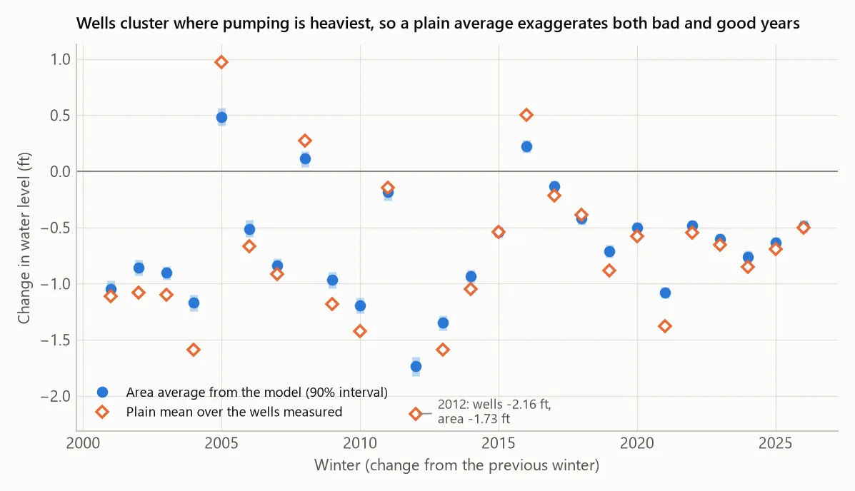
The DFC is defined over the aquifer, not over the wells, so the estimate needs a model that knows where the wells are and how much ground each one speaks for.
The first model failed
I wrote down the model and the tests it had to pass before fitting anything, because the easiest way to get a confident answer is to keep adjusting the model until it gives you one.
The first model gave each well its own level and a straight-line decline, with a spatial map of decline rates. It was fitted to 2000-2019 and asked to forecast 2020-2026 at the same wells. It lost to the dumbest forecast I could think of (last reading plus the average annual change) by 38%.
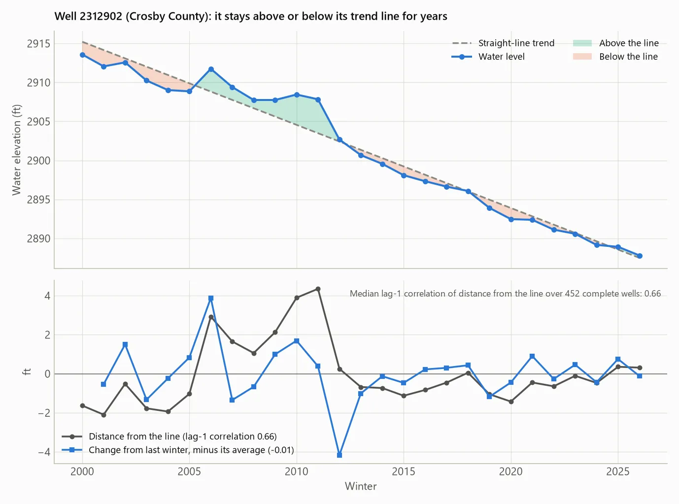
A likely reason showed up in the residuals. A well that sits above its own trend line one winter tends to sit above it for years (lag-1 autocorrelation 0.51). The model treated each winter’s deviation as fresh information, so it was overconfident about every one of them. Year-to-year changes barely correlate (-0.16), so I rebuilt the model around changes.
The replacement says a well’s change between two winters is its local decline rate, plus that year’s regional signal (wet years and dry years, which hit different parts of the area differently), plus noise with heavy tails so that a bad reading cannot drag the answer around. The decline-rate map and the yearly patterns are Gaussian processes; the whole thing is fitted in PyMC and sampled with nutpie in about an hour on a laptop. The area-average decline comes from posterior draws on a 5 km grid, which corrects for most of the clustering.
Checking the model against its own data
A model that forecasts well can still be wrong in ways that matter, so the next step was to make it simulate the data it was fitted to and look for differences from the real thing. Most of the picture came back right. The year-to-year regional signal was reproduced, and the residuals in the five winters that make up the headline number sum to almost exactly zero.
One thing came back wrong. The model had a single noise level for every well in every year, and the data don’t. The scatter between wells’ year-to-year changes was about 2 to 2.5 ft in the 2000s and has been 1.2 to 1.8 ft since about 2014. It is also larger in the southern counties than around Lubbock. With one noise level, the model’s intervals were too narrow before 2014 and in the south (covering 77-83% of changes in Martin, Garza, Dawson, Howard and Gaines, where they should cover 90%) and too wide recently.
My first guess was a change in how wells are measured. The districts moved from steel tape to electric line around 2014. That doesn’t seem to explain it: before 2014, changes measured with electric line were no less noisy than those measured with steel tape.
So I refitted the model with a noise level that drifts from winter to winter and differs by groundwater district. “Noise” here means everything the model doesn’t explain. That includes reading error, but also things like a neighbour’s pump running the week of the measurement.
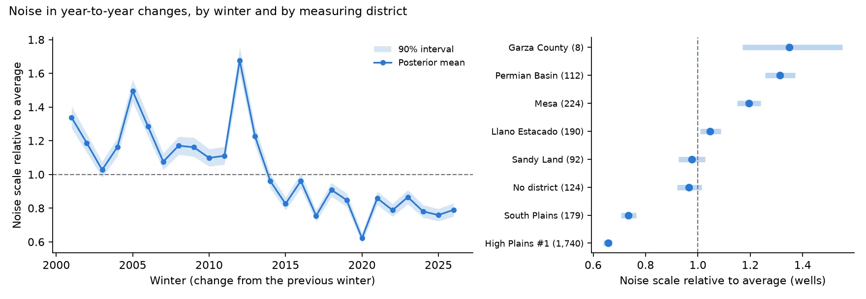
The fitted noise is about a third lower since 2014 than before. The spike in 2012 lines up with the change across the record 2011 drought, when it looks like some wells dropped far more than their neighbours. By district, wells measured by the High Plains Underground Water Conservation District, which runs about two-thirds of the network, scatter about half as much as those in Permian Basin and Mesa to the south. I don’t know why the scatter dropped after 2014, or how much of the difference between districts is measurement practice and how much is geology and pumping. Those are questions for the people who run the networks.
On the in-sample measures, the refit is better. Its leave-one-out predictive score (PSIS-LOO) improved by 1,745 ± 64 log units across 45,101 changes, and its intervals now cover about 90% in every period and 88-91% in the southern counties that were the worst before. The headline number moved by 0.03 ft. It does not fix everything. Large drops are more common than large rises in the real data, which a symmetric error distribution can’t reproduce. The model still expects a little more scatter than there has been in the last few years, and Lynn County is now slightly undercovered (83%).
This change was made after I had seen the results, which is exactly the kind of change the up-front design was meant to prevent, and it shows. Every improvement above is measured on the data that prompted the change. On the one forecast window I had held back (2014-2019), the refit actually scores about 2% worse than the original, though its intervals are better calibrated. So I can say the new model describes the data better, but not that it predicts better. Both versions are kept, with the first model’s results archived next to the second’s. The headline call is the same under both. Of the county calls, only Gaines differs, which is a good reason not to lean on any county that sits near its line.
There is one honest way to settle which model predicts better: data neither model has seen. On November 14, 2026, before anyone had measured a well for winter 2027, I had both models and four simple baselines forecast the winter-2027 water level in 1,923 wells. I committed the forecasts with a checksum, along with the scoring rules. The measurements come in over December to March and reach the state database by mid-2027. Then we’ll know.
How many wells does it take?
Because the whole network was measured every winter, there is a clean experiment available. Replay the winters from 2006, and each winter let a strategy pick which N wells to “measure”, using only what it knew from earlier winters. Feed the model those wells’ real readings and see how close the end result comes to the answer from all wells.
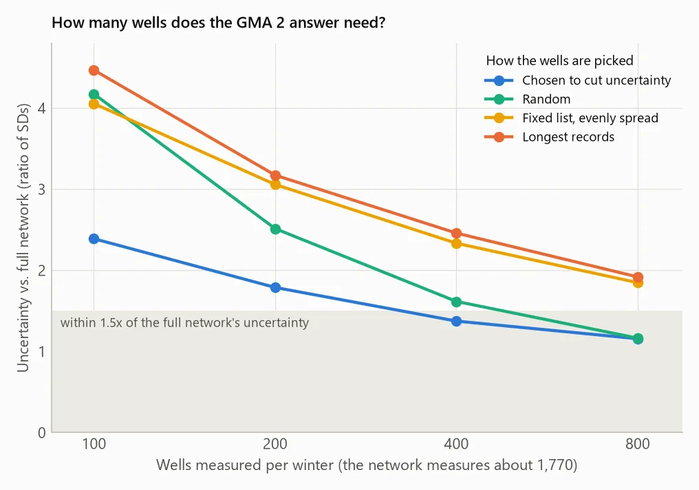
The first thing the replay shows is that the call itself is cheap. With 100 wells a winter, about 6% of the network, every strategy except pure random sampling reproduces the on-path call in every replicate and every winter, and none misses the five-year decline by more than half a foot. With a full foot between the estimate and the schedule, that is plenty.
Precision is what costs wells. Getting the uncertainty within 1.5 times what the full network gives takes about 400 wells a winter if they are chosen to cut uncertainty, or about 800 picked at random. Choosing wells for the uncertainty they remove clearly beats random sampling at 100 wells (by 0.11 ± 0.04 ft of error) and modestly at 400, ties at 200, and is slightly worse at 800, where random has already covered the ground.
That result depends on the noise model. Under the first model, which treated every well as equally noisy, the chosen wells never beat random on accuracy. Once the model knows that some districts’ wells scatter twice as much as others, it can steer measurements toward the quieter ones, and that is where the gain comes from.
One strategy is worth avoiding. Measuring only the wells with the longest records, which is a natural way to trim a network, biased the answer low by 0.2 to 0.45 ft in every budget. The likely reason is survivorship: a well only builds a long record if it hasn’t gone dry, so the long-record wells lean toward places where the decline has been slower.
The full network measures about 1,770 wells a winter. For the district-wide question alone, the replay suggests far fewer would do. I don’t think that is an argument for cutting it. County questions, local permitting and the wells people drink from need the density, and the replay only asks about one number.
What doesn’t hold up
The replacement model passed the forecast test on 2020-2026, beating the best simple forecast by 14%, with 90% intervals that covered 91% of outcomes. That test window had been seen before the model was rebuilt, though, so I held back a second one. Fitted to 2000-2013 and asked to forecast 2014-2019, it failed. It was good one and two years out and worse than “no change” four to six years out. Declines roughly halved after 2013, with wet winters in 2015-2017, and a model that treats each year’s weather as independent probably can’t see a multi-year wet spell coming. The headline number doesn’t rely on forecasting, since it estimates 2021-2026 from readings taken in those winters. But I wouldn’t use this model to say where the aquifer will be in 2030, and the monitoring-budget results above should be read as provisional for the same reason.
Between wells, the model adds less than you’d hope. Holding out 50 km blocks, its predictions of a well’s year-to-year change beat a plain “this winter’s average elsewhere” by only 4%. Most of a single well’s annual change is local. What the model contributes is the area weighting and an honest interval on the area average, not sharp predictions at places nobody measured.
There are three caveats I can’t close from public data. The DFC is defined over the active cells of the state’s groundwater availability model, and I averaged over the Ogallala outline in the 23 counties instead. The DFC is itself a model output, compared here with measured levels, which is what the districts’ own monitoring comparisons do, but it is not the same thing. And some wells stop being measured because they go dry. Continuing the falling trend of the 182 wells that dropped out of the network, a deliberately pessimistic assumption, raises the five-year decline from 2.98 to 3.24 ft, still well inside the schedule.
The districts have their own comparison, a 2026 technical memo cited in the DFC report as having “demonstrated the feasibility of achieving the desired future conditions”. That agrees in direction with what I found, but the memo isn’t posted, so I couldn’t compare numbers. I’d like to.
The same problem, in rocks?
Mineral exploration interests me because, from the outside, it looks like a cousin of this problem: something underground you can’t see directly, measurements that tend to cluster where someone already expected to find something, and a limited budget for more data. I don’t know that field well, and I’m sure it has complications groundwater doesn’t, so I won’t claim much here. But I’d like to find out how well approaches like the ones in this post carry over: writing the tests down first, checking the error structure before trusting an interval, and asking how much data a decision needs before asking where to collect it. That’s a project for another day.
Sources
- Texas Water Development Board, Groundwater Database
- GMA 2 desired future conditions explanatory report (2026 draft)
- High Plains Underground Water Conservation District, annual average changes (news releases)
The code, the full results, the design with its pass/fail criteria and the blind 2027 forecast are on GitHub.