Two answer keys, two winners: mapping Texas lakes from space
A deep-learning model against a one-line water index on the Texas Highland Lakes, scored against an AI's labels and my own.
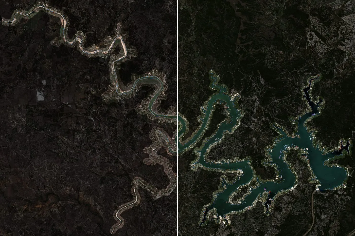
Explore the interactive map. Code and data on GitHub.
Most of my geospatial work is vector: parcels, infrastructure, networks, boundaries, the things you draw. Rasters I’ve mostly used as a backdrop. This project was a way to learn remote sensing properly by building something end to end, so every baseline got the same tuning rules as the model, and the losses are reported as plainly as the wins.
I built a deep-learning model to map Texas reservoirs from satellite images, and pitted it against the classic one-line method, a water-index threshold. To judge them I made two answer keys for the same 660 test points: one labelled by an AI model, the way a lot of labelling gets done now, and one labelled by me, blind. Then I scored every method against both.
The two keys agree on 97 % of the points. They still crown different winners. Scored against the AI labels, the deep model and one index (MNDWI) are neck and neck, and the other index (NDWI) looks like the worst method in the project. Scored against my labels, NDWI is the most accurate method I tested. The other 3 % of points, almost all at the water’s edge, decide the ranking.
That turned into the thread of the whole project: how much the answer depends on what you score against. Here is the setting.
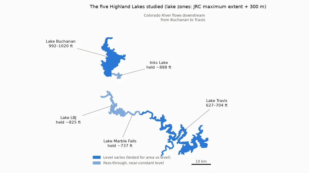
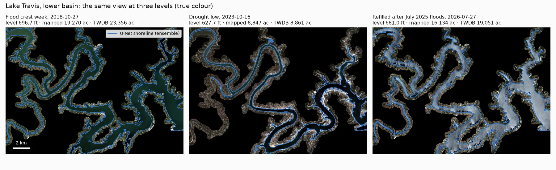
Lake Travis is a good stress test for anyone who maps water from space. In October 2018 a flood pushed it to 704 ft above sea level. Five years later, in the 2023 drought, it was down to 627 ft and had lost more than half its surface. By July 2025 it was full again. Upstream, Lake Buchanan swung 28 ft. LBJ, Inks and Marble Falls, the pass-through lakes between them, are held almost level the whole time. And the Texas Water Development Board (TWDB) publishes every lake’s level every day, so there is an official record to check the maps against.
The questions:
- Can a deep-learning model, fine-tuned from public pretrained satellite weights, map these lakes better than a water-index threshold?
- Can radar (Sentinel-1), which sees through cloud, fill the gaps that cloud leaves?
- Does the mapped area track the official lake level?
- Does any of it work on water nobody gauges, from small reservoirs down to stock tanks?
Everything is public: Sentinel-2 and Sentinel-1 from Microsoft’s Planetary Computer, JRC Global Surface Water, ESA WorldCover, Impact Observatory land cover, TWDB’s daily lake records, and USDA NAIP aerial photos for the stock tanks. It all ran on one desktop GPU.
The short version
- The answer key decides the per-pixel winner. Against my labels, NDWI with a cutoff near zero beats the U-Net (IoU 0.994 vs 0.968). Against the AI labels, NDWI comes last (0.80), because the AI marked 99 shoreline points “unsure” and those points drop out of the scoring.
- On lake area, NDWI (with the cutoff from my labels) ties the model. Both track the official level at r = 0.99 on the big lakes.
- The model earns its place where nothing simple works: radar (a cloud-proof monthly record, trained with no radar labels), an uncertainty map that flags its own errors, and a small edge on small, muddy reservoirs it had never seen.
- Where it fails: stock tanks of an acre or two, where plain NDWI found four times as many ponds, and a habit of drawing each lake’s usual outline.
- I’d deploy: NDWI on clear days, the radar model through cloud, and a hand-labelled answer key to check both.
The setup
Each lake gets a zone: the 1984–2020 maximum water extent from JRC, cut at the dams and widened by 300 m. The baselines are the two classic water indices, NDWI (green vs near-infrared) and MNDWI (green vs short-wave infrared). Each gets a cutoff tuned on hand-labelled points from the other lakes, and each is also run with a cutoff picked automatically per image (Otsu’s method).
The deep model is a U-Net whose ResNet-18 encoder starts from the SSL4EO-S12 MoCo weights in TorchGeo. It is trained on weak labels (more below), never on Travis when Travis is being tested, never on Buchanan when Buchanan is being tested, and only on 2018–2023 scenes. The radar model is a U-Net with a ResNet-50 encoder from SSL4EO-S12 Sentinel-1 weights. It learns to reproduce the optical model’s maps on days when a clear optical image and a radar pass are within two days of each other and the lake level barely changed.
There are two tests. One is 660 stratified points on 18 scenes, each judged by eye, twice (two answer keys, below). The other is a timeline of every usable date compared with the official record.
Here is the swing from orbit: the same 21 × 15 km window of lower Lake Travis at the 2018 flood, the 2023 drought low and after the 2025 refill. The blue line is the model’s shoreline.
Two answer keys
To score per-pixel accuracy you need points where you know the answer. I sampled 660, mostly in the band of shoreline the lakes move through, and labelled them from 400 m image chips in true colour and in a short-wave-infrared false colour, where water is unmistakably dark.
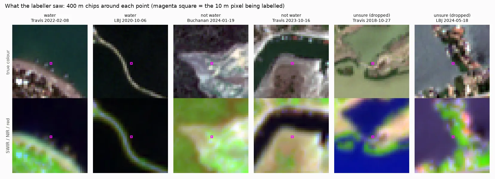
Every point was labelled twice, on purpose. AI-assisted labelling is fast and increasingly common, and I wanted to know whether an AI’s labels would give the same verdict as a person’s. An AI model (Claude Opus 5.5) labelled the points first, from the same chips. I labelled them second, in a small browser tool that never shows anyone else’s answer, so I couldn’t be swayed by it.
We agree on 97 % of the points we both committed on. The big difference is commitment: the AI marked 99 points “unsure”, almost all on the exact shoreline. I marked 20. Unsure points are dropped from scoring, so the AI’s caution removes the hardest pixels: exactly the ones where methods disagree.
To check myself, I re-labelled the 26 points where we disagreed, shuffled blind among 26 we agreed on. None of the controls flipped. Of the conflicts, I kept 17, moved 7 to unsure and switched 2 to the AI’s answer. My labels are the primary reference; the AI’s are kept and every method is scored against both, so you can see what each key says.
Round one: per pixel, the one-liner wins
On 585 held-out points (lakes and years the model never trained on):
| IoU | 95 % interval | |
|---|---|---|
| NDWI, tuned cutoff (≈ −0.03) | 0.994 | 0.987–1.000 |
| NDWI, Otsu cutoff per image (no labels) | 0.993 | 0.985–1.000 |
| S2 U-Net, 3-model ensemble | 0.968 | 0.952–0.983 |
| MNDWI, tuned cutoff | 0.939 | 0.904–0.968 |
Scored on the same points, NDWI beats the U-Net by 0.026 (interval 0.011 to 0.042), and by 0.038 on the strictest subset, a lake the model never saw in years it never saw. The U-Net is probably ahead of MNDWI (+0.029), but that interval just touches zero.
So the trained model loses per pixel to (green − nir) / (green + nir) with a cutoff near zero. The AI answer key tells a different story: there NDWI comes last of the main methods (0.80), because tuning on those labels pushes its cutoff to 0.23, where bright, turbid water falls just below it. With labels that commit on the shoreline, the best cutoff is near the textbook zero, and NDWI barely makes a mistake. Same images, same methods, 97 % agreement between the keys, and the ranking flips.
Part of NDWI’s win is what the test rewards. Each label judges one 10 m pixel, usually at the water’s edge. NDWI uses only 10 m bands. MNDWI and the U-Net also lean on 20 m short-wave infrared bands, and the U-Net looks at neighbouring pixels too. At a sharp edge, the sharpest method wins. That’s a real strength, but it isn’t the same thing as measuring a lake.
The U-Net’s misses are telling. Of the 22 points where it and NDWI disagree, NDWI is right on 19. They fall into two groups: lakebed that is usually under water but was dry that day, which the model still calls water, and water in places that are usually dry (the 2018 flood, the 2026 refills), which it misses. Both pull towards the lake’s usual outline. More on why below.
Round two: measuring the lake
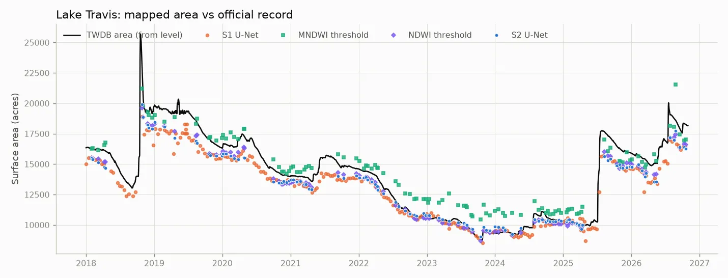
Pixel accuracy at random points is not what anyone wants from a lake map. They want the area, date after date. So I mapped every clear Sentinel-2 day (up to 2 per month) and every Sentinel-1 pass from 2018 to October 2026 and compared the mapped area with TWDB’s.
| r with lake level | error vs official area | error after a linear fit | |
|---|---|---|---|
| Travis (121 clear dates) | |||
| NDWI, tuned cutoff | 0.994 | 892 acres | 328 acres |
| S2 U-Net | 0.990 | 1,014 acres | 364 acres |
| MNDWI, tuned cutoff | 0.972 | 1,044 acres | 727 acres |
| ESA’s own SCL water class | 0.975 | 1,602 acres | 741 acres |
| Buchanan (148 clear dates) | |||
| NDWI, tuned cutoff | 0.993 | 992 acres | 211 acres |
| S2 U-Net | 0.992 | 925 acres | 213 acres |
| MNDWI, tuned cutoff | 0.993 | 1,017 acres | 235 acres |
The “after a linear fit” column removes any constant difference between what a method counts as lake and what TWDB’s rating curve counts, so it measures how faithfully each method follows the ups and downs. On that measure NDWI and the U-Net are tied at Buchanan, and NDWI is slightly ahead at Travis. MNDWI’s misfits at Travis swing with the lake itself: too much water in the low-water years, too little after the refill. No single cutoff suits both.
To see where NDWI and the U-Net differ, I mapped the date with the biggest gap between them:
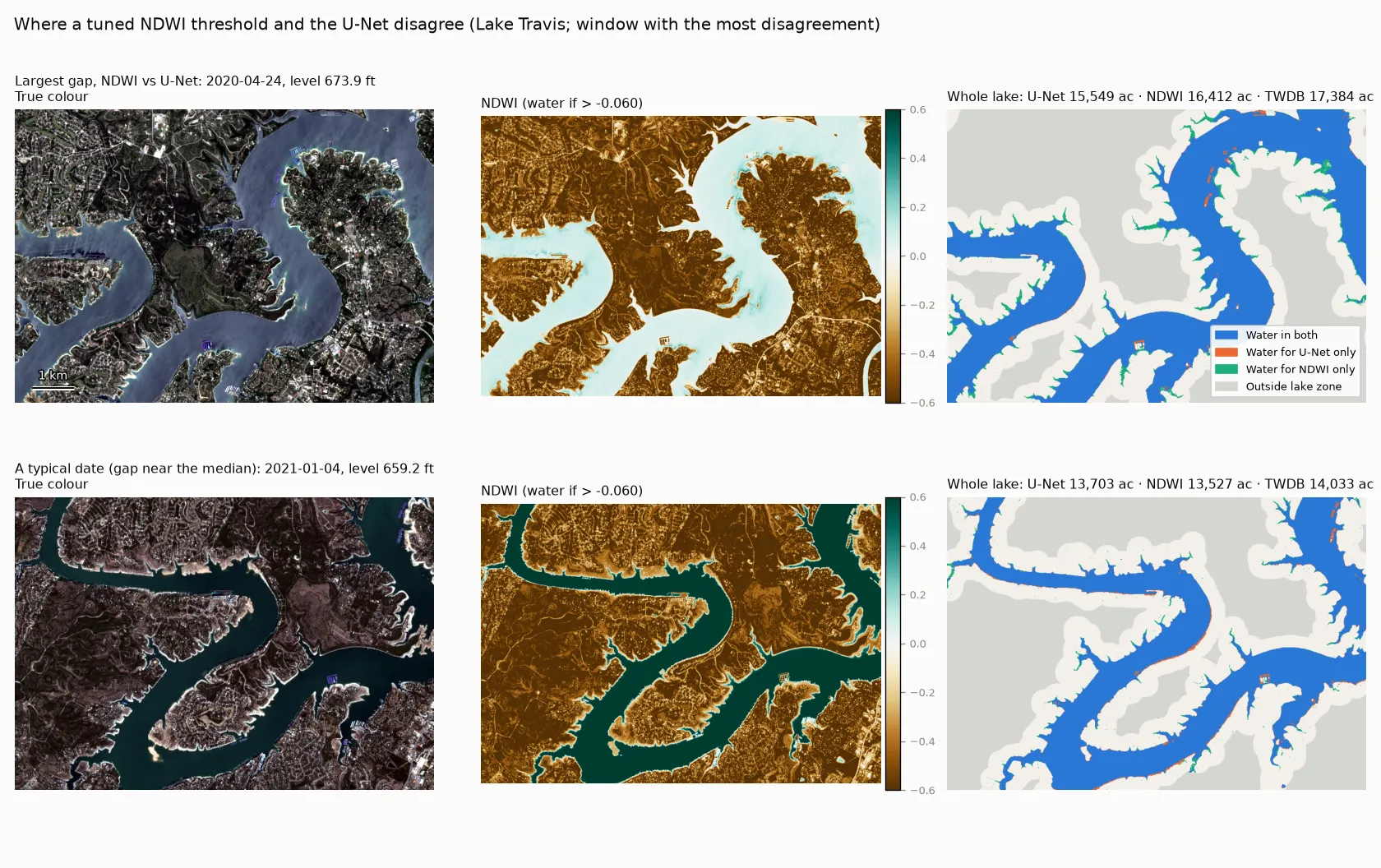
It’s a hazy spring day, and NDWI over the open water is barely above its cutoff. Still, NDWI picks up the narrow tips of the coves (green), which the U-Net smooths away. The U-Net’s only extra “water” is docks and boats (orange). Seeing a 2.5 km window of context is a strength for a blurry radar image. At a crisp 10 m shoreline it’s a small handicap.
The pass-through lakes: not quite a flat line
I meant LBJ, Inks and Marble Falls to be a noise floor: lakes held at near-constant level, where a good mapper should report a flat line. They turned out to be more interesting than that.
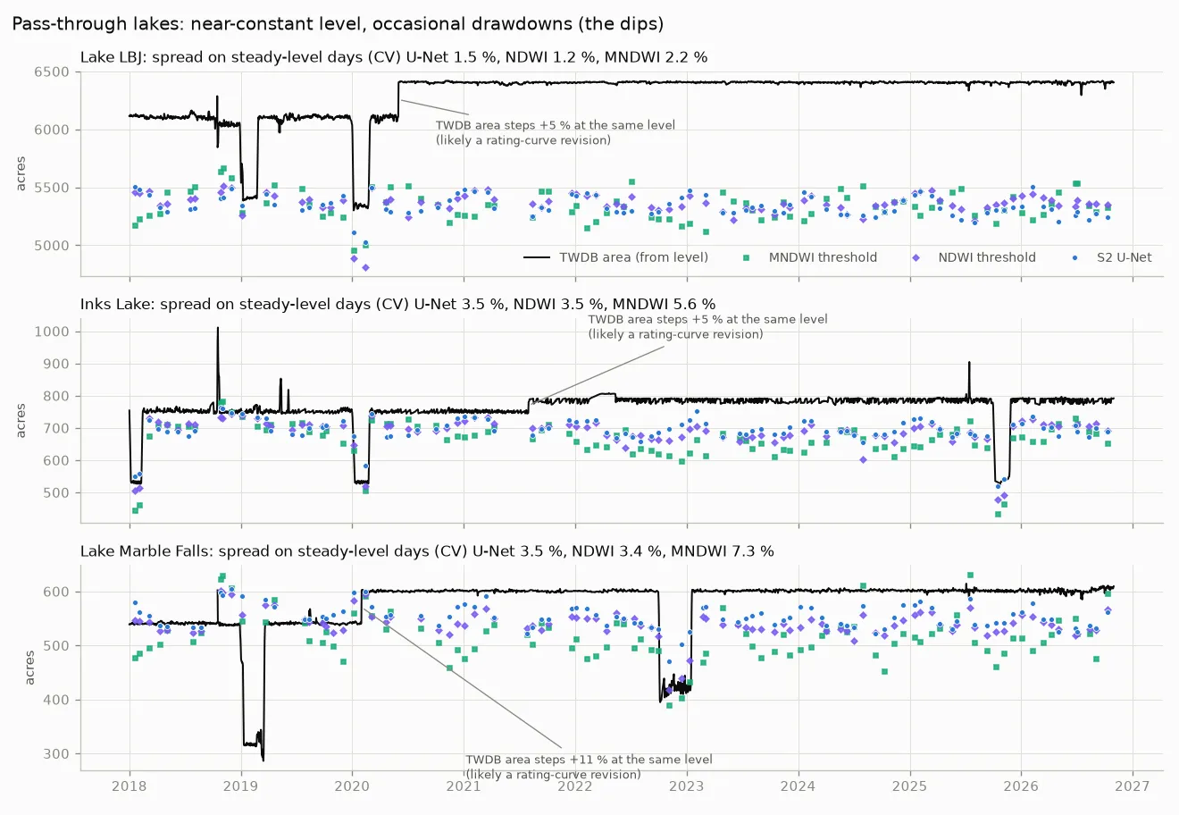
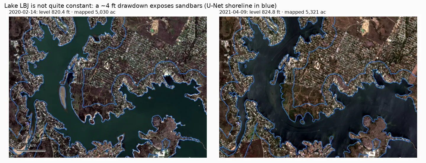
First, they are not constant. Each was drawn down a few times (4–8 ft for one to four months; the dips in the black line), and the imagery shows it plainly:
Second, TWDB’s official area steps up with no change in level: +5 % at LBJ in 2020, +5 % at Inks in 2021–22 and +11 % at Marble Falls in 2020. That looks like rating-curve revisions after new bathymetric surveys (I haven’t checked TWDB’s survey dates). The satellite record has no such step, a reminder that “official area” is a model too.
Taking only days when the level really was steady (within 0.5 ft of normal), the spread in mapped area is the noise floor proper. During the drawdowns, the question is how much of the official drop each method shows:
| Steady-day spread: LBJ / Inks / Marble Falls | Drawdown change: LBJ / Inks / Marble Falls | |
|---|---|---|
| TWDB area (from level) | — | −14 % / −28 % / −27 % |
| NDWI | 1.2 / 3.5 / 3.4 % | −7 % / −24 % / −13 % |
| S2 U-Net | 1.5 / 3.5 / 3.5 % | −4 % / −19 % / −6 % |
| MNDWI | 2.2 / 5.6 / 7.3 % | −5 % / −28 % / −15 % |
| S1 U-Net (radar) | 2.3 / 3.6 / 6.9 % | −4 % / −23 % / −15 % |
NDWI and the U-Net are equally steady when nothing is happening. But when the lake drops, the U-Net shows the least of it: 6 % at Marble Falls, against an official 27 %. Freshly exposed lakebed is wet, dark mud, and the U-Net keeps calling it water for a while. That’s the same lean towards the usual outline that the hand labels caught. There are only 3–6 optical drawdown dates per lake, but radar shows the same pattern.
Round three: radar through cloud
Central Texas is not that cloudy, but the cloud arrives with the storms, which is when lakes change fastest. With clear optical days only, Travis had a usable map in 70 % of months.
The radar model never saw a hand label. It was trained to reproduce the optical ensemble’s map on days when an optical and a radar image were taken within two days of each other and the lake level hardly moved. On the hand points it scored IoU 0.948, about 0.02 below the optical model and 0.08 above a tuned radar-backscatter (VV) threshold (95 % interval +0.03 to +0.13). The threshold is the classic radar water method, and it struggles here because wind-roughened water and smooth bare ground overlap in backscatter.
Over time it does better still. On all ~250 radar dates per lake, the S1 model’s area tracks level at r = 0.988 at both Travis and Buchanan. On dates with no clear optical image within three days, its median error against the official area is 3–7 %. The optical model on cloudy days is off by a median of 10–12 % with clouds left in, and by 30–36 % if you mask the clouds out (masking removes water along with cloud). Optical plus radar gives a usable map in 100 % of months.
The worst case shows why. On 3 February 2023 a deck of broken cumulus covered three quarters of Lake Travis. The optical model, shown an image of cloud tops, called almost the entire lake zone water: 45,401 acres, more than twice the lake’s full-pool area. Radar the next morning saw straight through:
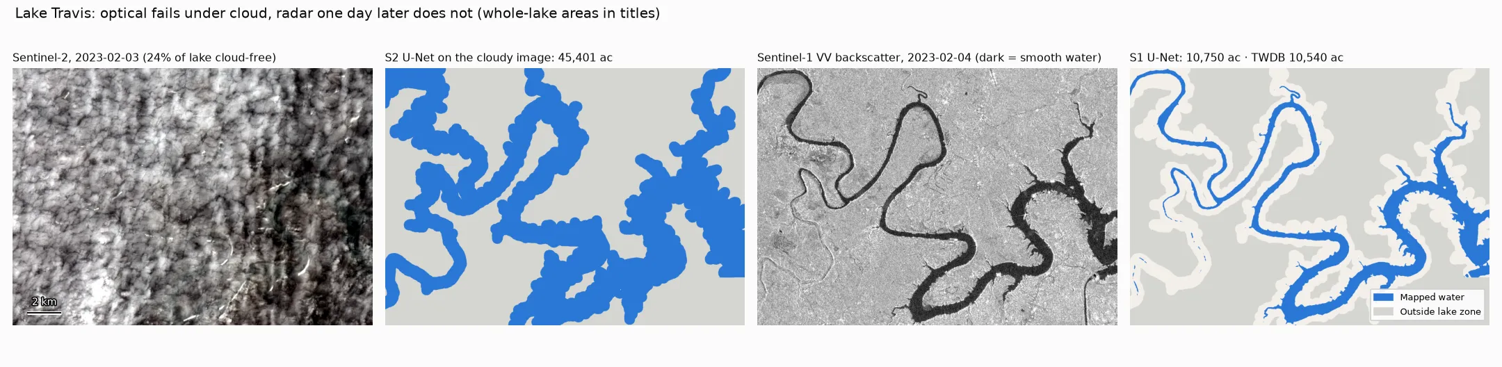
The radar model mapped 10,750 acres against TWDB’s 10,540. In the VV backscatter image (third panel) calm water is dark because it reflects the radar pulse away from the satellite. That simple physics is what the VV-threshold method relies on. The threshold breaks down when wind roughens the water or smooth bare ground looks just as dark: its area tracks level at only r = 0.91 at Travis and 0.57 at Buchanan, against 0.99 for the radar U-Net, which uses context as well as brightness.
This is the part of the project I’d actually deploy, and it’s where the deep model clearly earns its keep. No index exists for radar that works this well, and teaching the radar model from the optical one needed no radar labels at all.
Where weak labels mislead
Nobody has drawn water masks for these lakes, so the model has to learn from labels that are cheap and wrong in known ways. I scored five candidates against the hand-labelled points before training anything (the numbers below use my final labels). That turned out to be the most useful hour of the project.
| Weak label | What it is | IoU vs hand points | Precision | Recall |
|---|---|---|---|---|
| JRC occurrence ≥ 50 % | Landsat water frequency 1984–2020, one static map | 0.78 | 0.86 | 0.90 |
| ESA WorldCover 2021 | One static land-cover map | 0.81 | 0.86 | 0.94 |
| Impact Observatory annual | Land-cover map per year (2017–2023) | 0.83 | 0.93 | 0.89 |
| Sentinel-2 SCL water | Per-scene class from ESA’s L2A processor | 0.94 | 0.97 | 0.96 |
| SCL ∩ JRC history (used) | SCL water, ignored where JRC never saw water | 0.94 | 0.97 | 0.96 |
The static maps look excellent in a screenshot, and on a lake that holds its level they are nearly right. On a reservoir that moves they fail in three specific ways:
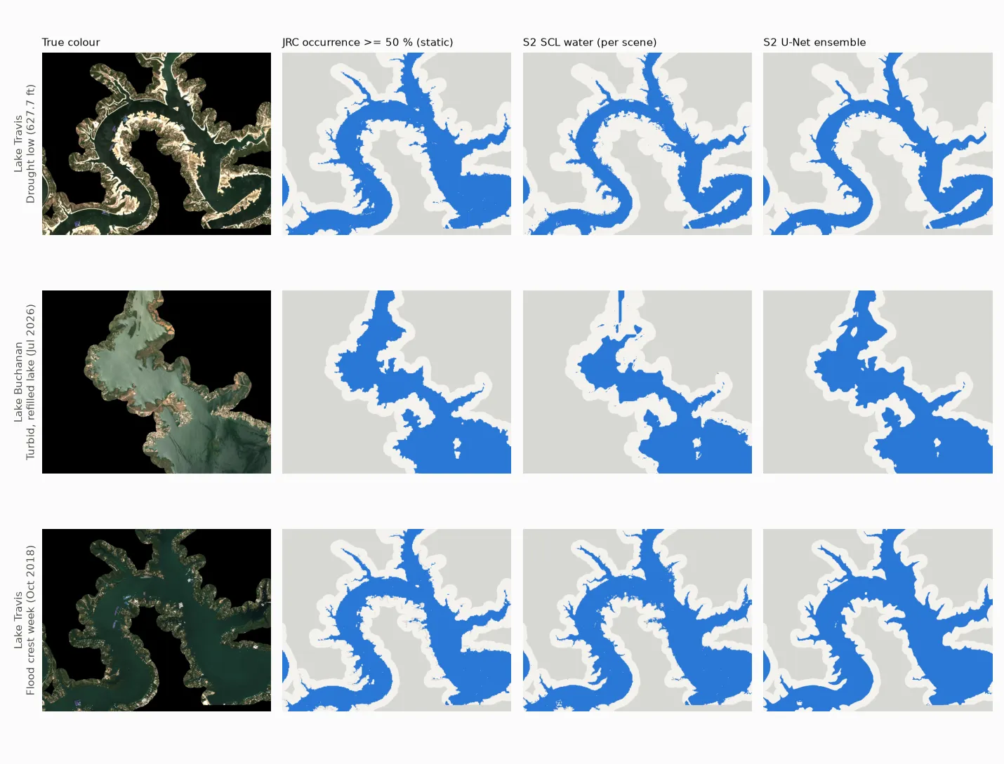
1. They paint the dry lakebed as water. In October 2023 and January 2024, with the lakes near their lows, the static JRC and WorldCover masks marked 13–20 of the dry points on each Travis and Buchanan scene as water. Those were exposed mud and scrub where the lake usually is. A model trained on those labels learns that “a usual lake location” means water. The ablation shows the cost: the same U-Net trained on JRC ≥ 50 % instead of per-scene SCL scored 0.78 on held-out points, against 0.96 for the SCL-trained model on the same points.
2. They miss water that is only there sometimes. The October 2018 flood scene at Travis had 12 water points that JRC’s majority map calls dry. A frequency map says nothing about the week the lake was 23 ft above normal.
3. “Annual” is not current. Impact Observatory’s map is updated every year, which sounds like it should fix both problems. It stops in 2023, though, and the lakes refilled in 2025. Using the most recent map for 2026 scenes missed 16 water points per Buchanan scene.
The per-scene SCL class avoids all three, because it is computed from the same image. I combined it with the JRC history (“ignore SCL water where JRC has never seen water”) to throw out river glint and stray ponds. In hindsight, that combination is probably where the model’s pull towards the lake’s usual outline comes from. The JRC part of the label carries the lake’s history, and the model learned some of it. A model can partly outgrow its labels, but its leftover errors tend to sit where the labels were biased.
Two smaller lessons:
- Check labels against independent truth before training. The ranking of weak labels by agreement with the hand points (0.78 → 0.94) predicted the ranking of the models trained on them.
- Ignore is a label. Cloud, shadow, and SCL water in places JRC has never seen water are set to ignore, not land. It costs nothing and removes the most confident wrong labels.
Does the model know when it’s wrong?
I tried two uncertainty methods: a deep ensemble (three seeds) and MC dropout (ten stochastic passes through one model). This is something the index can’t do at all: a threshold gives no hint of where it’s unsure.
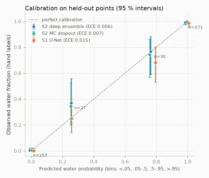
Both are well calibrated (expected calibration error 0.006–0.007). That number is flattering on its own, because almost every point gets a probability near 0 or 1 and is right. The 57 points in between are the real test, and here the two answer keys differ. Against my labels the ensemble is close to honest: points it scores at about 0.27 are water 37 % of the time; points at about 0.78 are water 77 % of the time. Against the AI labels, far fewer points land in the middle (29 against 48 in the same bins), because the AI left most of them unsure, and the few that remain look over-confident (calibration error 0.011 against 0.006). Calibration is judged on exactly the pixels a cautious labeller skips.
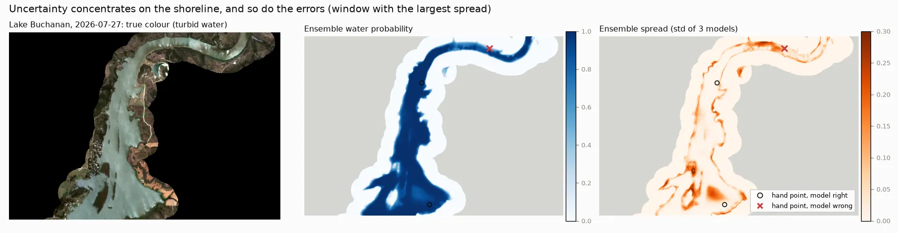
The more useful test is whether disagreement picks out the errors. It does. The ensemble’s standard deviation ranks wrong points above right ones with AUROC 0.95 (MC dropout: 0.94). In the web app this is the orange band along the shoreline: it marks where the map should not be trusted, and it is almost always a few pixels wide.
Round four: small reservoirs it never saw
The Highland Lakes are gauged every day. On those lakes a satellite map mostly confirms the gauge. The place it would be worth having is a reservoir without one. A truly ungauged reservoir has nothing to score against, so I used the next best thing: ten small West and Central Texas reservoirs that do have a TWDB record, mapped as if they didn’t.
They were picked by fixed rules from TWDB’s list of 122: maximum area between about 300 and 7,000 acres (Mackenzie is barely 1 km² of water), an area swing of at least 45 % since 2018, a complete record, and a setting unlike the training lakes (red-clay turbid water, shallow mudflat basins, narrow canyons). No retraining, no fine-tuning. The index and radar cutoffs are the ones tuned on the Highland Lakes, and TWDB’s numbers were opened only to score the result.
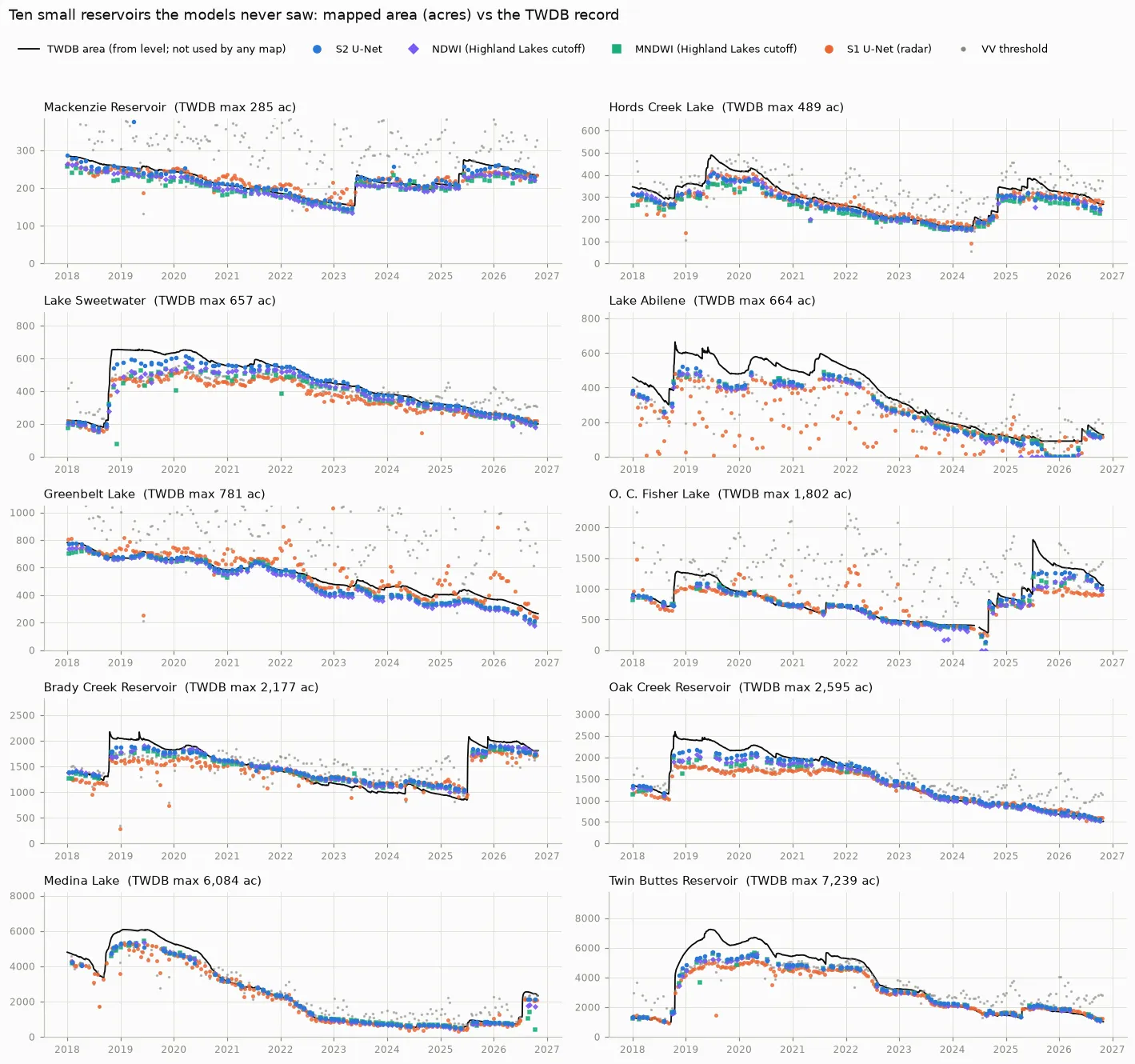
On a lake with no gauge you can’t calibrate, so raw error is what a user would get:
| median across 10 lakes | raw error | median signed error | error after a linear fit |
|---|---|---|---|
| S2 U-Net | 6.0 % | −2 % | 5.6 % |
| NDWI, Highland Lakes cutoff | 7.5 % | −7 % | 6.8 % |
| MNDWI, Highland Lakes cutoff | 8.1 % | −7 % | 7.7 % |
| S1 U-Net (radar) | 11.0 % | −7 % | 13.9 % |
| VV threshold (radar) | 20.9 % | +6 % | 22.1 % |
Here the model finally has an edge, though a modest one:
- It depends on size. The U-Net and NDWI split the ten lakes 5–5 on raw error. On the five smallest, though, the U-Net is closer to TWDB than NDWI on most dates (84–100 % of dates at four of them). On the four largest, NDWI is closer on most dates. NDWI’s under-count grows as lakes shrink, because a fringe of mixed shoreline pixels is a bigger share of a small lake.
- Muddy floodwater. After Medina refilled in July 2026, TWDB put it at about 2,500 acres. The U-Net mapped about 2,140, NDWI about 1,750 and MNDWI anywhere from 400 to 1,400.
- Tracking. After a linear fit (a diagnostic, since it needs a gauge), the U-Net follows the ups and downs better than NDWI on 8 of 10 lakes, and better than MNDWI on 9 of 10.
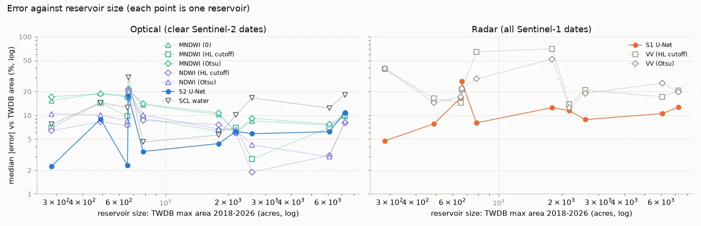
Radar beat the VV threshold on 8 of 10 lakes, and with it every month has a map. But it is noticeably weaker on small lakes than on the big ones: correlation with TWDB 0.71–0.97, against 0.99 at Travis. Use optical when it is clear and radar to fill the gaps.
Two honest caveats. Lake Abilene is 17–21 % low for the U-Net and both indices, all at high water, which points at flooded vegetation or the rating curve rather than at any one method. And everyone under-maps high water: on six of the ten lakes the U-Net’s mapped swing is only 68–87 % of TWDB’s, and the indices fall about as short.
Round five: stock tanks nobody gauges
Texas has hundreds of thousands of stock tanks and farm ponds, mostly a few acres or less, and nobody records their level. With no gauge to borrow, I used a sharper eye instead: USDA’s NAIP aerial photography, flown over Texas every two years at 0.6 m with a near-infrared band. A 1-acre pond is about 11,000 NAIP pixels and 40 Sentinel-2 pixels. On each flight date I outlined water from the photo and compared it with satellite maps from the nearest days.
The reference took more work than the test:
- Shadow strips. The first water rule outlined tree shadows along every creek, so ponds now need a compact core.
- Plowed fields. In two 2022 flights, plowed fields came out as water. NAIP isn’t calibrated, and bright bare soil passed the index, so water now also has to be far darker in NIR than in red.
- A refinery. One site landed on a refinery whose shadows looked like ponds. Built-up land is now masked, and that site was moved to brush country.
Then 60 random reference outlines were checked by eye. The AI assistant went first and doubted 17 of them, mostly the smallest ponds. I then checked the same 60 blind, in a small browser tool, and found 59 plainly water and one I couldn’t call (a pond half-hidden by sun glint). So the reference holds up down to the smallest ponds; the doubt was the AI’s, not the photo’s. Same pattern as the two answer keys, in miniature. The scores still use ponds of a quarter-acre or more, because that is about ten Sentinel-2 pixels and below it every method mostly misses.
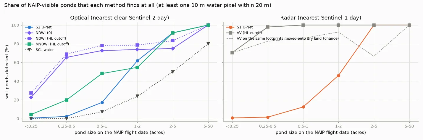
The trend from the reservoirs reverses sharply. On 461 ponds at eight sites:
| ponds ≥ 0.25 acre | found | found by chance | total area vs photo |
|---|---|---|---|
| NDWI, Highland Lakes cutoff | 74 % | 0 % | −40 % |
| MNDWI, Highland Lakes cutoff | 37 % | 0 % | −53 % |
| S2 U-Net | 19 % | 0 % | −58 % |
| S1 U-Net (radar) | 16 % | 1 % | −51 % |
| VV threshold (radar) | 99 % | 85 % | −1 % |
The “by chance” column matters. I moved every pond’s footprint about 650 m onto dry land and ran the same test. The radar threshold “found” 85 % of those empty footprints, so its 99 % is almost all speckle.
NDWI finds more ponds than the U-Net at 6 of 7 sites and ties at the seventh. The U-Net catches up only above about 2 acres. For a pond five pixels across, it produces a faint, smooth blob that rarely reaches 0.5. It learned water from lakes tens of pixels wide.
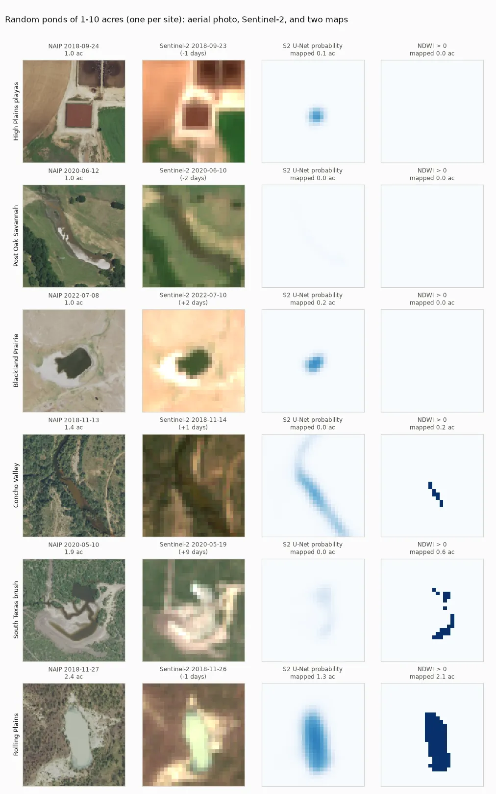
Even the winner misses about 40 % of total pond area, because about half of a small pond’s pixels touch the bank. At this size, satellite “area” is a wetness index, not acreage. NAIP would make a ready source of pond labels for anyone who wants to train a model that does better.
What I’d tell someone starting this
- Start with NDWI and a cutoff near zero. It is free, explainable, and per pixel it beat my model. Try Otsu’s automatic cutoff too; it did just as well.
- Your answer key is part of the result. A cautious labeller who drops the hard pixels makes every method look better and hides real differences. Here, switching answer keys turned the worst baseline into the best. If you use AI labels, score against a hand-labelled set too, and give yourself a blind second look.
- Evaluate on the quantity you care about, and on more than one regime. Per-pixel accuracy, lake area over time, steady lakes, small lakes and ponds each told me something the others didn’t.
- Look at the errors. My first explanations for several gaps were wrong until I mapped where the methods disagreed.
- Audit weak labels against a small, independent labelled set before training. It took an hour, it predicted which training runs would work, and it explains the model’s main bias.
- Use the deep model where nothing simple works. For me that was radar: a model taught by the optical maps beat the radar threshold on almost every test, and it fills every cloudy month. Its uncertainty map is the other thing no index gives you.
- Test one scale further than you planned. On reservoirs of a few hundred acres, the model edged out the index. On one-acre stock tanks, the index found four times as many ponds. “It generalises” always comes with a scale attached.
- Pretraining helped less than I expected. MoCo SSL4EO weights beat random initialisation by +0.003 IoU, well within noise. With hundreds of scenes and an easy target, the label source mattered far more.
The interactive map
Everything above is browsable in a small web app: pick a lake, drag a slider between the low-water and high-water images with the mapped shoreline and the uncertainty band on top, and see mapped area against the official record over time, with NDWI as an optional series. A second row of tabs covers the ten small reservoirs. It is a static page with no libraries, so it loads fast and costs nothing to host.
Limitations
- One labeller. The primary labels are mine, made carefully and checked with a blind second look, but they are one person’s calls on hard shoreline pixels. The per-pixel ranking differs between the two answer keys; treat it as specific to this labelling.
- TWDB “area” is level passed through a rating curve, not a measurement. The curve counts flooded trees, sub-pixel coves and the lake zone definition in ways a 10 m pixel can’t see, and the curves are occasionally revised. Correlation with level is the robust measure; absolute acres are not.
- The U-Net leans towards each lake’s usual outline. It is slow to call freshly exposed lakebed land and slow to call new floodwater water. Anyone using it to monitor lakes that move a few feet should calibrate for this, or retrain with labels that don’t carry the JRC history.
- Radar learned from optics, so it inherits optical errors, and it was not separately tested on windy days or flooded vegetation.
- One region. The transfer and pond tests add ten reservoirs and eight pond sites, all in Texas. The stock-tank reference is one aerial snapshot per site every two years, checked by eye rather than surveyed. Treat the effect sizes as indicative.
Code, data snapshots and weights: GitHub (MIT). Interactive map: alo.mn/apps/mapping-texas-lakes-from-space/. Contains modified Copernicus Sentinel data 2018–2026.